2 Language modeling: the basics
This chapter covers
- The basics of language modeling
- How to build the simplest possible (but functional) language model
- How traditional, statistical language models work
- Why and how \(N\)-gram language models improve upon statistical models
- Strategies to evaluate language models in a principled way
We saw in Chapter 1 some of the amazing things large language models can do; we learned about different types of LMs, transformers, and we saw that they can be used as a “base layer” for any NLP task.
Let’s now dive deeper into language modeling as a discipline and cover the basics, such as the origins of the field, what the most common models look like, and how one can measure how good an LM is.
Neural LMs are also a big part of language modeling, but they will be covered in ?sec-ch-neural-language-models-and-self-supervision — many important details justify us dedicating a chapter to them.
In Section 2.1 we will see an introduction to language modeling and explain how the need to model language first appeared. In Section 2.2 we will show with code and examples what the simplest possible language model could look like. Section 2.3 and Section 2.4 introduce Statistical and \(N\)-gram models, respectively, including worked examples for both types of models. Finally, we explain how to measure a given LM’s performance in Section 2.5.
2.1 Overview and History
As explained in the previous chapter, a language model (LM) is a device that understands how words are used in a given language.
Practically, it can be thought of as a function (in the computational sense) that takes in a sequence of words as input and outputs a score representing the probability that the sequence would be valid in a given language, such as English.
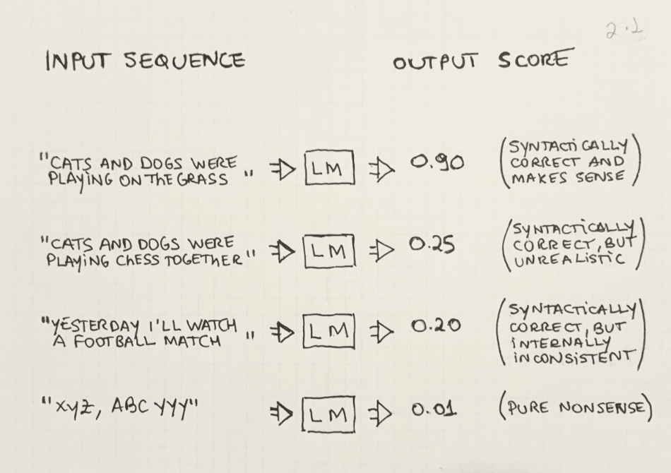
The definition of valid may vary but we can see some examples in Figure 2.1 below. Intuitively, the sentence “Cats and dogs were playing on the grass” would be considered valid in the English language: it gets a high score from the LM. Examples (2), (3), and (4) show several ways in which a word sequence may be considered invalid, or unlikely according to an LM. Examples (2) and (3) don’t make semantic sense (even though all individual words exist). Example (4) is made up of words that don’t exist, so it gets a low score from the LM.
In addition to being able to score any sequence of words and output its probability score, LMs can also be used to predict the next word in a sentence. An example can be seen in Figure 2.2 in the next Section.
The next section explains why the two basic uses (scoring and predicting) are two sides of the same coin and why the distinction between training-time and inference-time is so important for LMs.
2.1.1 The duality between calculating probabilities and predicting the next word
As we said before, the uses for a language model are:
- Calculating the probability of a word sequence
- Predicting the next word in a sentence
These two use cases may seem unrelated but 1 implies 2. Let’s see how.
Suppose you have a trained LM that can calculate the probability of arbitrary sequences of words and you want to repurpose it to predict the next word in a sentence. How would you do that?
A naïve way to predict the next word in an input sequence would be to generate all possible sentences that start with the input sequence and then calculate the probability of every one of them. Then, just pick the variation that got the highest probability score and the word that generates that variation as the chosen victor.
This strategy is shown in Figure 2.2: We start with the sentence “A dog was running on the ______” and then we generate multiple variations having multiple filler words in the missing space and score each variation with the LM—to pick the highest score.
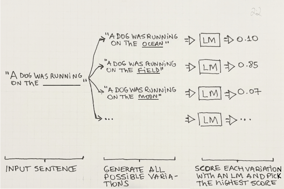
In short, if you have a function that outputs the probability score for a sequence of words, you can use it to predict the next word in a sentence—just generate all possible variations of the next word, score each one, and pick the highest-scoring variation! This is why scoring and predicting are two sides of the same coin—if you can score a sentence, you can predict the most likely next word in it.
This brute-force approach is not often used in this manner in practice, but it helps understand the relationship between the two concepts. We will revisit this duality in Section 2.3.1 when we present yet another way to look at this problem, from the prism of conditional probabilities.
The language models we will focus on in this book learn from data. This is in contrast with systems that are built off expert knowledge, which are sets of hard rules manually created by human experts.
You are probably aware that there exists an actual branch of science that deals with such data-driven systems; it’s called Machine Learning (ML). All language models we will study in this book are machine learning models. This means that most concepts, terms, and conclusions from the ML world also apply to language models.
The concepts of training-time and inference-time are core to machine learning. Let’s explain them from the prism of language models.
At training-time, the language models are trained on the training data. How this training is performed will depend on the specific model type used (statistical LMs, neural LMs, etc), but regardless of the specifics of the algorithms used, they all share this concept of learning from data.
After the model is trained we can proceed to the inference-time. This refers to the stage at which we use (or perform inference with) the model. The model can be used in one of the two ways we have already mentioned: calculating the probability of a word sequence or predicting the next word in a sentence.
Figure 2.3 provides a visual representation of these two concepts. On the left, an LM is trained with a set of documents (the corpus), and on the right, we see one example of the inference-time use of the model.
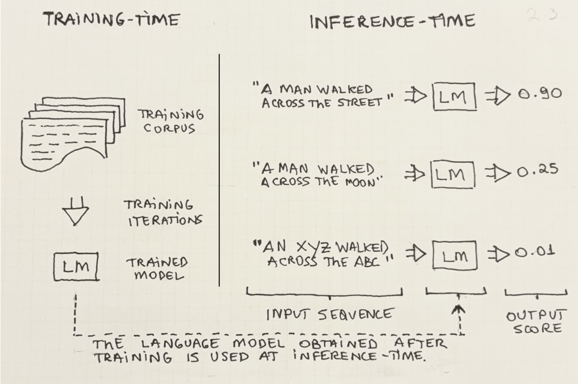
Remember, everything the language model knows was learned at training-time. When the model is used at inference-time, no new learning takes place—the model simply applies whatever knowledge it learned previously.
The distinction between train and inference-times is also critical to the way we evaluate models. Regardless of the evaluation technique we use, we must never evaluate a model on the same dataset it was trained on. Measuring performance on a different set (so-called test set) is a basic tenet of machine learning. We will cover simple ways of evaluating LMs in Section 2.5.
Language modeling as a concept is not a recent discovery, by any means. Its origins trace back to the early 20th century, as we will see next.
2.1.2 The need to model language
The need to model language had already been identified as far back as the 1940s. In the seminal, widely-cited work “A Mathematical Theory of Communication” (Shannon (1948)) we see early formulations of language models using probabilities and statistics, in the context of Information Theory.1
1 Information theory studies how to transmit and store information efficiently
As we saw earlier, a simple way to think of a language model is as a function that takes in a sequence of words and outputs a score that tells us how likely that sequence is in a given language.
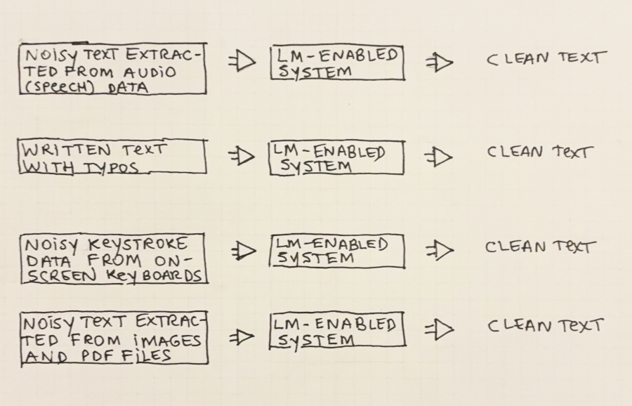
In addition to all NLP use-cases we will see later in the book, several real-world scenarios benefit from such a simple function. Let’s see some examples below. These are summarized in Figure 2.4:
Speech Recognition: Speech-to-Text or Voice-typing systems turn spoken language into text. Language models are used to help understand what is being said, which is often hard in the presence of background noise.
For example, if the sound quality is bad and it’s unclear whether someone said “The dog was running on the field” or “The dog was running on the shield”, the former is probably the correct option, as it’s a more likely sentence than the latter. An LM is exactly the tool to tell you that.
Text correction: Many people have trouble spelling and using words correctly. Language models are also helpful here as they can detect misspelled words—by simply validating every word again a list of known words. They can also be used to inform users when words and sentences are not being used correctly.
For example, the sentence “Last week I will go to the movies” is grammatically correct, but a good LM can detect that it contains a mistake, as it’s using a verb in the future with an adverb in the past.
Typing Assistant (on-screen keyboards): Mobile phones with on-screen keyboards can benefit from language models to enhance user experience. Keys are delimited by small areas on the screen and users often type as fast as they can, touching the screen imprecisely and making typing mistakes. LMs can be used to correct text on the fly.
For example, “i” and “o” are close together in a standard English-language QWERTY keyboard. Therefore, if a user types something that looks like “O went to the movies” in an on-screen keyboard, a language model can easily figure out that this is a mistake and correct it to “I went to the movies”, which is a much more likely sequence.
Extracting text from images (e.g. OCR): Extracting text from images and other types of binary files such as PDF is helpful in many settings. People need to scan documents and save them as text; cameras and software need to extract text from videos and/or static images.
Data in other media types (audio, image, video, etc) is inherently lossy and noisy—think of a picture of a car’s license plate, taken at night under low lights—so it’s useful to have some means to calculate how likely some text is so that you can trust your readings.
We have so far seen how LMs work and we also saw that they can be used in one of two ways: scoring and predicting. We understood the difference between training and using these models, and some real-life scenarios where they could help. Let’s now see what it would take to build a very simple—the simplest possible—LM in the next section.
2.2 The simplest possible Language Model
Let’s think about what the simplest possible language model would look like. Any ideas? What would you say is the simplest way to describe a language such as English?
We can say that a language is simply the collection of every word in the training corpus. It sounds very simplistic (and it is), but let’s use this as an example to help illustrate how we would build and use such a language model.
2.2.1 Worked Example
Let’s see some examples of how this would work in practice:
Training-time
For our simplest possible LM, training consists of going through every document in the training corpus and storing every unique word seen. For this example, our training corpus will consist of a single document, containing 39 tokens (including punctuation):
“A man lives in a bustling city where he sees people walking along the streets every day. The man also has a home in the country, but he prefers to spend his time in the city.”
Listing 2.1 shows a Python snippet that could be used for training our “simplest possible” LM:
simplest_possible_lm = set() # empty set

corpus = ["a", "man", "lives", "in", "a", "bustling",
          "city", "where", "he", "sees", "people",
          "walking", "along", "the", "streets", "every",
          "day", ".", "the", "man", "also", "has", "a",
          "home", "in", "the", "country", ",", "but", "he",
          "prefers", "to", "spend", "his", "time", "in",
          "the", "city", "."]

# training: just loop over every word in the corpus
# and add them to a set
for word in corpus:
    simplest_possible_lm.add(word)
For this simplest possible LM, training consists simply of collecting all unique words in the training set.
Ok, so what exactly do we do with this information? How does one go about using this simple language model? Like any other LM: assigning probability scores to arbitrary word sequences.
Inference-time
We need to define how this model will score a sequence. Let’s say that a word sequence is deemed valid depending on how many valid words it contains. The score will therefore be the fraction of valid words in the sequence.
For example, if a sequence contains 4 words and 3 of them are valid words, its score is ¾ or 0.75. Let’s formalize this in Equation 2.1 below:
Listing 2.2 shows what the Python code would look like for the scoring at inference-time. Right now we assume that there are no duplicate words in the input sequence and that the sequence is non-empty.
How does our model know what a valid word is? It’s any word it’s seen in the training corpus.
In Figure 2.5 we can see 4 different word sequences and how they would be scored by our model. According to Equation 2.1 and following Listing 2.2, we have to count how many valid words there are in the sequence and divide by the total number of words.
Sequence (1) “A man lives in the city” is straightforward. All 6 words are known (i.e. they are part of the corpus the model was trained on) so it gets a perfect 1.0 score. With sequence (2) we see one shortcoming of our model: even though the input sequence doesn’t make sense it still gets a 1.0 score because the model only looks at words individually and ignores their context. Sequence (3) is again simple to understand: the words “xyz” and “yyy” are invalid because they are not part of the training corpus, so the sequence gets 4 out of 6 or 0.67 as a score. Finally, in sequence (4) all words are invalid, so it gets a zero score.
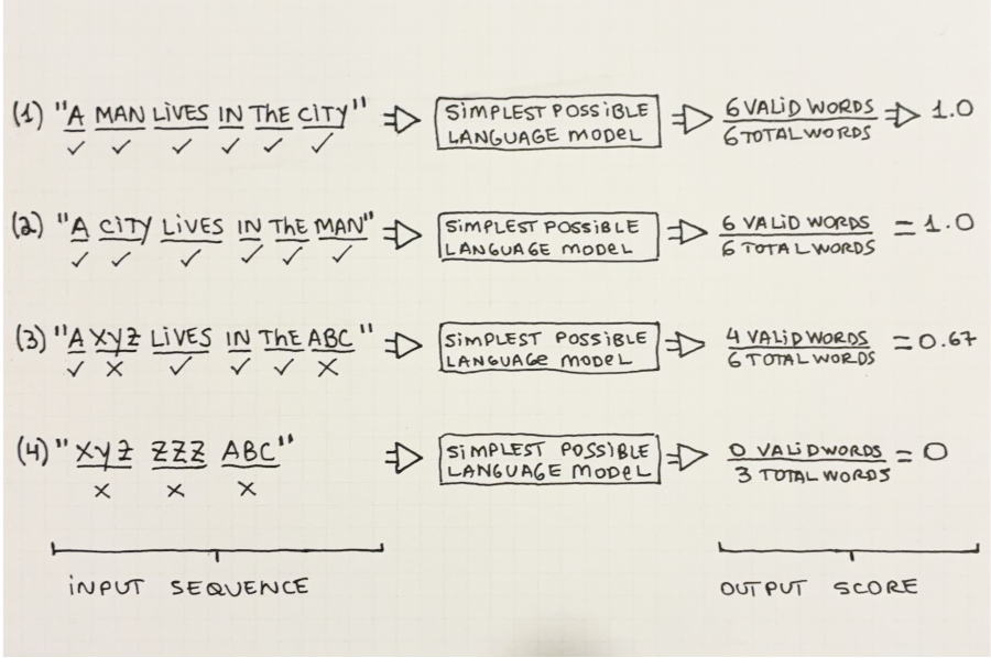
Figure 2.5 highlights one very important point that is true for all models we see in this book: Everything depends on what data the model has seen at training-time. We see a perfectly good sentence (example (3)) which received a low probability score because we used a very limited training corpus.
There is much more to language modeling than is seen in our “simplest possible” LM (or we wouldn’t need a book on the topic), but the basics are here: it can learn from text data and it’s able to score arbitrary word sequences. These two steps have been described in code, in Listing 2.1 and Listing 2.2, respectively.
Every other language model we will see in the book will be some variation of this basic strategy. Any method by which you can accomplish these two tasks (train on a corpus and calculate the probability of sequences of words) is a language model.
In this chapter we will analyze two such methods: Section 2.3 will cover statistical language models, which are perhaps the first nontrivial type of language model. Then, in Section 2.4, we will learn about \(N\)-gram models, which are an enhancement on top of statistical LMs.
2.3 Statistical Language Models
Statistical language models are an application of probability and statistical theory to language modeling. They model a language as a learned probability distribution over words.
In this book we focus on word-level language models, where the smallest unit considered by the model is a word. Most LMs we read about are word-level models but that doesn’t mean other types of models don’t exist. Character-level LMs are one such example.
In character-level LMs, probability scores are calculated for sequences of characters instead of sequences of words. Similarly, instead of predicting the next word in a sequence, they predict the next character in the sequence.
Character-level LMs do have some advantages over word-level models. Firstly, they don’t suffer from collapsing probabilities2 due to out-of-vocabulary words—the vocabulary for character-level LMs is just a limited set of characters.
Also, they are better able to capture meaning in languages with heavy declension and in-word semantics such as Finnish and German.
The reason why they aren’t as common as word-level LMs is that they are more computationally expensive to train and that they underperform word-level LMs for English, which is the language most applications are made for.
2 Situations where at least one of the composing terms of a conditional probability product is zero, thus causing the whole product to collapse to zero. A more thorough explanation can be seen in Section 2.3.2.
Let’s now see a practical explanation of statistical LMs, how they work, and go through a worked example. We’ll also cover their limitations—some of which will be addressed when we discuss \(N\)-gram language models in Section 2.4.
2.3.1 Overview
The goal of statistical language models is to represent a language, such as English, as a probability distribution over words. In this framework, a word sequence is deemed likely if it has a high probability of being sampled from that distribution. We can use it to define a function that takes a word sequence and outputs a probability score.
Even though the terms “probability” and “likelihood” are not exact synonyms in statistics literature, we shall use them as such to follow the convention in the NLP field. When the meaning is not clear from the context we will explicitly differentiate them.
But wait! Isn’t this similar to what we had previously, with our simplest possible language model? Yes, it is. The difference is how this function is built. In the case of statistical LMs, this function is a probabilistic model, learned empirically from counts and frequencies of words and sentences in the training corpus.
A statistical LM defines the probability of a sentence as the joint probability of its composing words. The joint probability of a sequence of words is the probability that all individual words appear in the training corpus, in that order.
In the next subsections, we show how to calculate the probability of a sentence. We must first learn how to calculate the probability of a single word; then we will see how to extend the calculation for full sentences. In Section 2.3.2 we have a fully worked example to see how statistical LMs work with real data, both at training- and at inference-time.
Probability of a word
Borrowing some notation from statistics and probability theory, \(P(''word'')\) represents the probability of a word. As with any probability, it must be a value between 0 and 1.3
3 Jurafsky and Martin (2025) is a great source for the more mathematically-inclined reader.
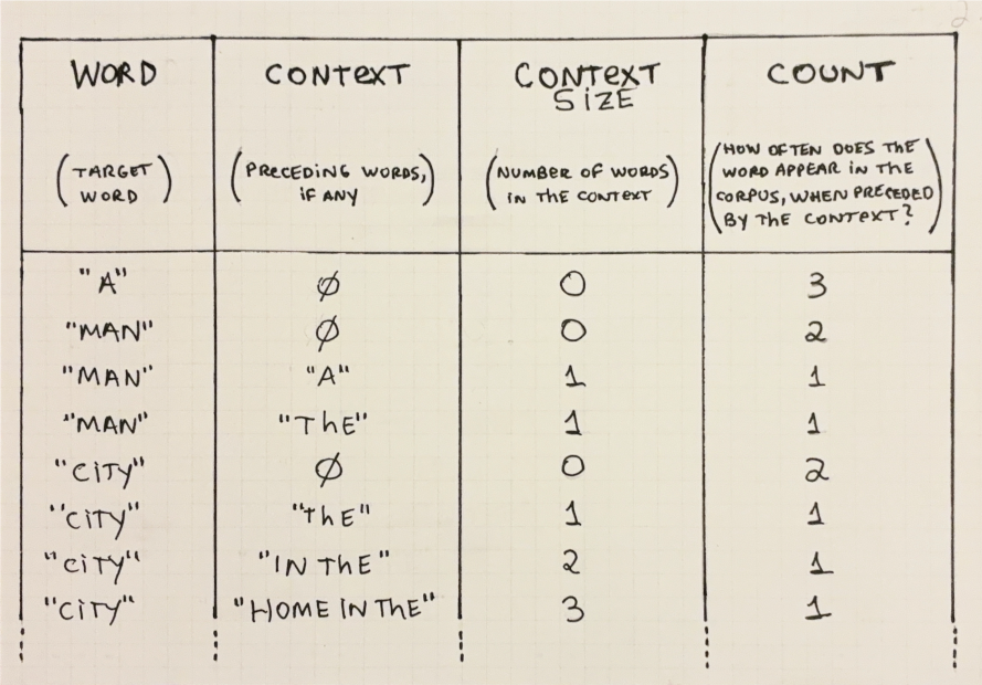
We calculate the probability of a single word by counting how many times that word appears in the training corpus and dividing by the corpus size. In other words, the probability of a word is its relative frequency in the training corpus. Figure 2.6 shows some examples of words and their probabilities, given some training corpus:
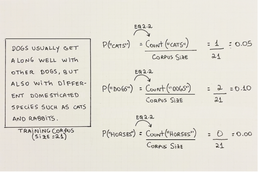
Let’s write down an informal formula for the probability of a single word in Equation 2.2:
Probability of a word preceded by some context
A word’s context are the words that precede it. This concept is very important and it will be key in several parts of this book.
The probability of a word in a context (represented by \(P(word\ |\ context)\))4 is a measure of how often that word is used after that context. This can be calculated by dividing the count of the full sequence by the count of the context on its own. Figure 2.7 shows an example of how to calculate this using a given corpus:
4 The symbol ‘\(|\)’ is read as “given” or “conditioned on” in statistics literature. When we are talking about text, however, it means “preceded by”. For example, \(P(''field''\ |\ ''a\ dog\ played\ on\ the'')\) should read: the probability of the word “dog” when preceded by the words “a dog played on the”.
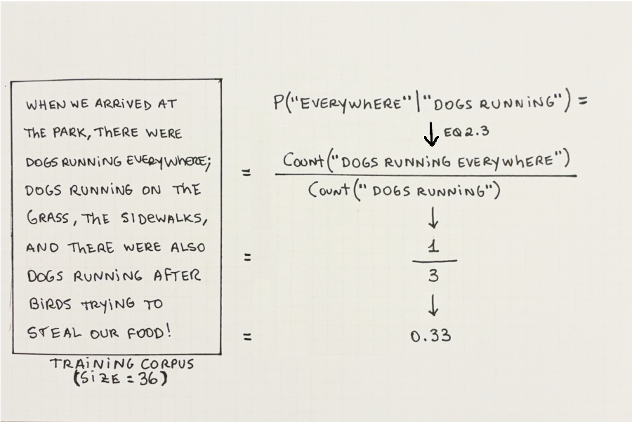
Equation 2.3 formalizes the calculation:
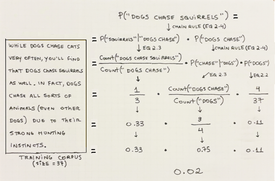
Probability of a sequence of words
Similarly to a single word, a sequence of words can also be represented as a probability, but a joint probability, which is the probability that every word in the sequence appears together, in that order.
The chain rule of probability (Equation 2.4) is a mathematical device that allows us to decompose a joint probability into a product of probabilities (each of which we can calculate with Equation 2.2 and Equation 2.3 above).
Figure 2.8 provides an example showing how the pieces fit together:
In Section 2.1.1 we showed the link between calculating the probability of a sequence of words and predicting the next word given a context. We mentioned that one could predict the most likely next word by a brute force approach; that is, generating all possible options for the word, calculating the probability for each variation, and picking the one with the highest score.
When we are talking about Statistical LMs there is another very clear link between calculating and predicting.
The chain rule of probability is a mathematical device that can be used to decompose a joint probability into a product of conditional probabilities.
If you have the individual conditional probabilities of every word in a sequence given a context, you simply need to multiply them to arrive at the full joint probability of the sequence.
While in ?sec-3-the-duality-between-calculating-the-probability-and-predicting-the-next-word we use a language model to calculate the probability for each variation of the sentence and pick the highest variation to predict the most likely next word. Here it’s the other way around: we use the probability of each possible variation to calculate the probability of the whole sequence.
Let’s look at a worked example in the next section.
2.3.2 Worked example
Let’s see how all these concepts tie together with a complete worked example. We’ll use our tiny training set so that calculations are simple and easy to understand. The examples at inference-time are carefully chosen so that we see the “happy path” but also some pathological cases to show the limitations of the model.
Training-time
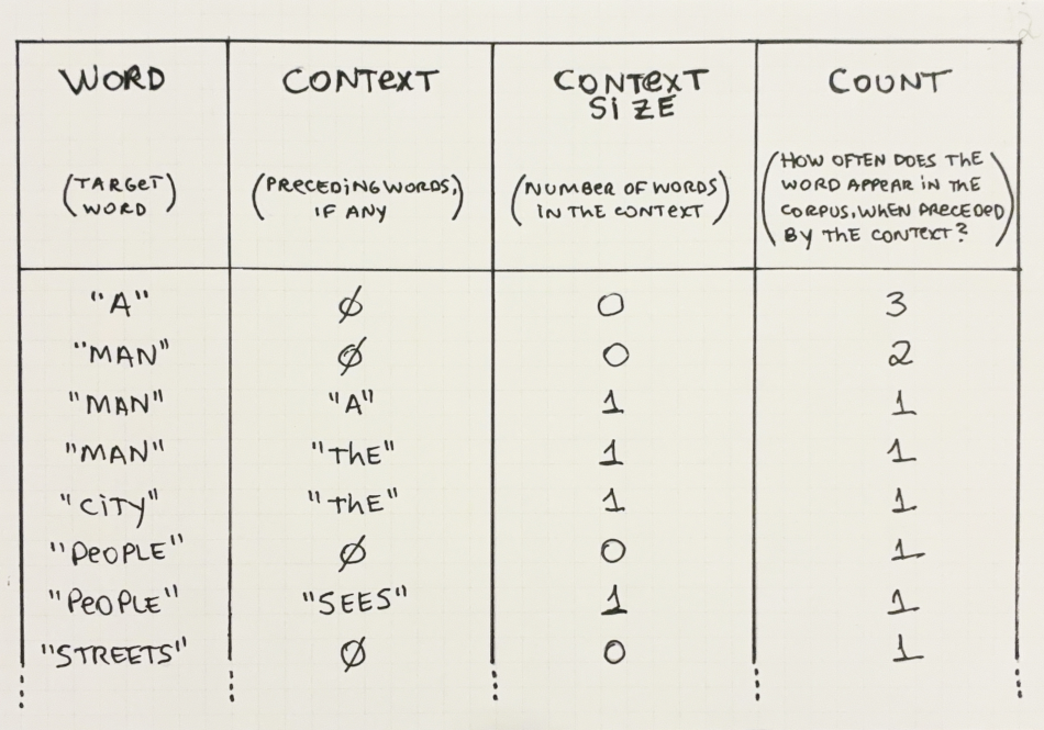
The first thing we need is a training set—a corpus of text to train the model on. Let’s use the same text we used earlier:
“A man lives in a bustling city where he sees people walking along the streets every day. The man also has a home in the country, but he prefers to spend his time in the city.”
We can represent the trained model with a table as Table 2.1 below.5
5 For simplicity’s sake, we will consider words in a case-insensitive manner. Only a few examples are included; the full table would be too large.
For a statistical language model, training refers to pre-calculating these probabilities and then storing them somewhere (e.g. in memory or on disk) for quick retrieval at inference-time.
Inference-time
With the model trained on the corpus above, we can simply retrieve the values to perform inference. Let’s see some examples:
Calculating the probability of the sentence “a man”:
For a short sentence like “a man”, the calculations are simple enough; we just need to decompose the joint probability into conditionals using the chain rule and then use the counts as calculated in Table 2.1.

Calculating the probability of the sentence: “a home in the city”:
This example shows the first failure mode of statistical LMs: the probabilities may collapse to zero if the model is asked to output the probability of a sentence it hasn’t seen in that exact order in the training set.
Calculating the probability of the sentence: “people running along the streets”:
In this example, the calculation also fails, because a single word (“running”) is absent from the training set. A single missing word “poisoned” the product and cause it to collapse to zero.
Figure 2.9 above shows a basic case where a statistical language model can provide an adequate probability score to an (admittedly short) phrase. Figure 2.10 and Figure 2.11 above were meant to display two limitations of statistical LMs, namely: the collapse of probabilities to zero, due to words that don’t appear in the training set in that order; the inability of these models to generalize to out-of-vocabulary words, even when they are semantically similar to other words found in the text.
When calculating the probability of a sequence, we arrive at figures such as 0.001, 0.3, 0.007, etc. We know that these numbers indicate how likely a piece of text is, as measured by a trained language model. But what does a value of 0.0002 mean as opposed to 0.00002 (which is ten times less likely)?
In practice, the nominal values don’t matter much at all. They only matter in a relative way when, for instance, a system is trying to decide which of two sentences provides the best completion for some user-entered text. In this case, the only thing that matter is their ordering.
Also, real-world systems apply many transformations and optimizations to these probabilities and may not even calculate them directly.
For example: many systems calculate sums of log-probabilities instead of products of probabilities, to promote numerical stability; It’s also common to normalize probabilities by the length of the sentence (otherwise shorter sentences are always going to be “more likely” than longer ones for simple numerical reasons). There are even mathematical shortcuts that allow one to calculate the ordering of values without needing to calculate the values themselves.
Let’s now summarize the limitations of statistical language models.
2.3.3 Limitations
The examples we just saw provided some hints why a naïve statistical language model can hardly be used in practice. It’s true that we used an artificially small dataset to train the model, but even if we train such a model on a very, very large corpus, it will never contain every possible sentence. And even such a corpus existed, there would be no hard-disk large enough to store all the necessary information.
Collapsed probabilities: A clear limitation of statistical LMs is that inference is based on multiplications of conditional probabilities.
When calculating probability for a sequence of words, if any of the conditional probabilities are 0 the whole product collapses to 0. This can be seen in Figure 2.10 and Figure 2.11. In Figure 2.10 all individual words were in the vocabulary, but not in that context, whereas in Figure 2.11 the product collapsed due to an out-of-vocabulary word (“running”) . Zero-valued probabilities are problematic because they prevent one from comparing the relative probabilities of two sequences.
Generalization: In Figure 2.11 we saw that we got a collapsed probability for the sequence “People running along the streets”, which is explained by the fact that the word “running” is not in the training set. Any conditional probability term that includes this word will collapse to 0.
A better model should be able to understand that the word “running” is similar to “walking”, which is a word that does appear in the training set. Being able to generalize—that is, transfer probability density—across similar words would make for a more useful model, as it would reduce the need for every possible sequence to be present in the training set.
Computational cost: Training a statistical LM like the one we used in the worked example means going over the training corpus and recording how often each word appears, in what context.
This may seem easy enough with a small train corpus (as used in the example) but what if we were to use a large corpus with a vocabulary containing 1 million6 terms? If we had to store the conditional probabilities of 1 million terms appearing in multiple contexts, the disk space needed would be prohibitively expensive, precluding any practical use.
6 1 million is the rough order of magnitude of the vocabulary size used in popular open-source NLP packages.
That’s it for the basics of statistical language models. In the following section, we’ll see what \(N\)-gram models are and how they help address some of the limitations seen above. Although \(N\)-gram models are an approximation to (or a subtype of) statistical LMs, they are different enough to merit their own section.
2.4 \(N\)-gram Language Models
In the previous section, we saw some of the limitations of statistical language models. These are mostly related to (a) the computational cost caused by the need to store a lot of information and (b) the inability of the model to generalize its knowledge to unseen word combinations, causing collapsing probabilities.
\(N\)-gram language models are more efficient statistical LMs and, at the same time, address some of their limitations. Let’s see how, starting with an explanation of what \(N\)-grams are.
2.4.1 \(N\)-grams
\(N\)-grams are a generalization over words. They can be used to represent single words but also pairs, triplets, and larger sequences thereof.
The choice of \(N\) in an \(N\)-gram defines the length of the smallest unit we use. For example, a 1-gram (also called a unigram) is an \(N\)-gram with a single element, so it’s just another name for a word. A 2-gram (also called a bigram) is simply a pair of words, whereas a 3-gram (also called a trigram) is an \(N\)-gram where \(N=3\), and it’s simply a sequence of 3 words—a triplet.
The actual term “\(N\)-gram” has been around for at least some decades, as it’s used in works such as those by Shannon (1948). In that specific work, however, character \(N\)-grams were used instead of word \(N\)-grams.
Let’s see how the same sentence would be represented using \(N\)-grams, with different values for \(N\). Figure 2.12 shows what the sentence “Cats and dogs make unlikely but adorable friends” looks like when split into uni-grams (\(N\)-gram with \(N=1\)), bigrams (\(N\)-gram with \(N=2\)), and trigrams (\(N\)-gram with \(N=3\)).
We can leverage \(N\)-grams to create approximations of fully-fledged statistical language models. Let’s see how and why \(N\)-gram models tend to work better in practice.
2.4.2 \(N\)-gram models explained
\(N\)-gram models are an approximation of a full statistical language model. They operate under two assumptions:
We don’t need to know all the previous words in the context—just the last \(N-1\) words;
The closer a context word is to the target word, the more important it is.7
7 The last word before the target word is more important than the second-last word, which in turn is more important than the third-last word, and so on.
\(N\)-gram models work just like the models we saw in Section 2.3, with a subtle but key difference: The conditional probabilities obtained after decomposition are pruned after \(N-1\) steps. Following assumptions (1) and (2), we don’t need to consider all the context words to arrive at adequate estimations of probabilities—just the last \(N-1\), just like an \(N\)-gram of order \(N\). This greatly simplifies the calculations and helps avoid some problems as we will see in the examples.
In Figure 2.13 we see an example of how to calculate the probability of a sentence using an \(N\)-gram model with \(N=2\) (right side) and compare it to the way it’s done for a regular statistical LM (left):
\(N\)-gram models can be seen as the result of applying an engineering mindset to purely statistical LMs, which are a theoretical framework that provides a solid foundation to study language from a mathematical standpoint, but not very practical for real-world use.
\(N\)-gram models are not only more efficient than statistical LM but also provide better results in the presence of incomplete data. Let’s see some ways in which \(N\)-gram models are better suited to language modeling.
2.4.3 Advantages over Statistical LMs
Up until now, we saw how \(N\)-gram models are an efficient approximation to fully statistical LMs. It turns out there’s another benefit when we consider collapsed probabilities.
Efficiency: Statistical LMs and \(N\)-gram Models need to store conditional probability counts somewhere—either in memory or on disk—as they are trained. \(N\)-gram models require less space because the number of conditional probability combinations we need to keep track of is smaller (only contexts up to \(N-1\) need to be kept). In addition to that, inference is also faster, as the number of multiplications is smaller.
Reduced chance of collapsed probabilities: Since a smaller number of context words are taken into account when calculating probabilities, there’s a reduced chance of hitting upon a combination of words that were never seen in the training corpus. This means that there will be fewer zero terms in the conditional probability product—which in turn means that the result is less likely to collapse to zero.
2.4.4 Worked example
Similarly to what we did for statistical LMs in Section 2.3.2, let’s now see how we go from a body of text (the training corpus) to a trained \(N\)-gram language model, and see what results we get when we perform inference with it.
Training-time
Let’s use the same text again, to make comparisons easier:
“A man lives in a bustling city where he sees people walking along the streets every day. The man also has a home in the country, but he prefers to spend his time in the city.”
\(N\)-gram models only need to store the counts for a limited combination of contexts. For example, if we are using an \(N\)-gram model with \(N=2\) we only need to store the counts for words with up to 1 context word. This greatly reduces the amount of space needed.
Let’s see the information we would need to store, in Table 2.2 below. Note that in this table there are no entries for combinations where the context size is larger than 1.
Inference-time
Let’s see some examples of our \(N\)-gram model being used at inference-time:
Calculating the probability of the sentence “a man”:
For “a man”, the result is the same as we got in Section 2.3.2 for the example with statistical LMs. This happens because the sentence is so short that it makes no difference if we use the full context or just an \(N\)-gram.
Calculating the probability of the sentence: “a home in the city”:
Differently from the example for statistical LMs (Figure 2.10), the probability calculated by an \(N\)-gram model is non-zero because none of the terms collapsed to zero. This is one example where using an \(N\)-gram model instead of a statistical LM avoided collapsing probabilities.
Calculating the probability of the sentence: “people running along the streets”:
Several terms are simpler than the equivalent example calculated by the statistical LM in Section 2.3.2. However, the probability of the whole sentence still collapsed to zero because “running” is an out-of-vocabulary word.
Even though \(N\)-gram models have clear benefits over purely statistical LMs, they also have their own limitations, as we’ll see next.
2.4.5 Limitations
In the previous section, we saw that \(N\)-gram models fail to provide correct scores for relatively simple input sequences. Let’s analyze some of the main shortcomings of these models.
Limited context: Using a reduced version of the context increases efficiency and reduces the risk of collapsed probabilities. But in some cases—especially if one chooses a small value for \(N\)—there will be some loss in performance because relevant words will be left out of the context.
Let’s see an example with the following sentence: “People in France speak ______”.
As explained in Section 2.1, we can predict the most likely next word by generating all variations, calculating the probability score for them, and then picking the highest-scoring variant. Let’s analyze what these would look like when calculated using \(N=2\) and using \(N=3\).
Since we want to keep the example simple, we will only consider the scores for two variants: “People in France speak Spanish” and “People in France speak French”. A human would naturally know that the latter is the correct answer, but what would our model say?
We can see the difference in Figure 2.17 below. When we use \(N=2\), the model would assign almost the same score to both variants, so it will not be able to realize that “French” is a better candidate than “Spanish” for the missing word. Adding a single word to the context (increasing \(N\) to \(3\)) allows the model to include a new word and it makes all the difference. It’s now able to use conditional probabilities that include the word “France”, which naturally occurs much more often together with “French” than it does with “Spanish”!
Figure 2.17: A clear case where using an N-gram model with too small a context hinders performance. When we use \(N=3\), the model can pick up a context that includes the word “France”. Since the word “France” is used much more often with “French” than it is with “Spanish”, the model is more likely to infer that the missing word is “French”. EOS is a marker for the end of the sequence. The choice of \(N\) introduces a tradeoff between efficiency and expressivity; smaller values of \(N\) make the model faster and require less storage space but larger values of \(N\) allow the model to consider more data to calculate probabilities.
Collapsed probabilities: As we saw in Figure 2.16, \(N\)-gram models are still vulnerable to collapsed probabilities due to out-of-vocabulary words. It’s not as vulnerable as pure statistical LMs, but the issue persists.
Generalization: With respect to generalizing to semantically similar words as those seen at training-time, \(N\)-gram models don’t help us much in comparison with regular statistical models.
We saw an example in Figure 2.16. Even though the calculations were simpler and faster, we again hit upon a collapsed probability—and the model wasn’t able to transfer probability from the word “walking” to the word “running”. The generalization problem will be solved with Neural LMs and Embedding Layers, which will be discussed in ?sec-ch-neural-language-models-and-self-supervision.
Some of these limitations were worked around—or at least mitigated—with a little engineering ingenuity:
2.4.6 Later optimizations
\(N\)-gram models are an optimization on top of regular statistical LMs, but they fall short of a perfect model. Additional enhancements were proposed to make \(N\)-gram models more capable and address some of their limitations. These include backoff, smoothing, and interpolation. Table 2.3 shows the main objectives of each strategy:
| Strategy | Objective |
|---|---|
| Backoff | Reduce the chance of collapsed conditional probability products |
| Smoothing | Reduce the chance of collapsed conditional probability products |
| Interpolation | Increase the quality of model output |
Let’s explain each in more detail.
Backoff: Backoff is a strategy whereby one replaces a zero-term with a lower-order \(N\)-gram term in the conditional probability decomposition—to prevent the whole product from collapsing to zero.
As an example, let’s calculate the probability score for the string “w1 w2 w3 w4” using backoff and \(N=3\). If the word “w4” is never preceded by “w2 w3” in the training set, the conditional probability \(P(''w4''\ |\ ''w2\ w3'')\) will collapse to zero, so we back-off to \(P(''w4''\ |\ ''w3'')\) instead. See Figure 2.18 for a visual representation.
Figure 2.18: If the term \(P(''w4''\ |\ ''w2\ w3'')\) has zero probability in the train set, a simple trigram model would cause the score for “w1 w2 w3 w4” to collapse to zero. Using a backoff model allows us to replace the zero-term with a lower-order \(N\)-gram instead, which can prevent the collapse at the cost of slightly lower accuracy. Smoothing: Smoothing refers to modifying zero terms in the conditional probability decomposition, to avoid collapsed probabilities.
The simplest way to do this is called Laplace Smoothing (aka Add-one Smoothing). It works by adding \(1\) to every \(N\)-gram count before performing the calculations. This will get rid of zeros and prevent probability collapse. See an example in Figure 2.19 below:
Figure 2.19: By adding \(1\) to every count before multiplying the terms, we get rid of zeros and we have a valid—non-collapsed—score. Interpolation: Unlike backoff and smoothing, interpolation is used to enhance the quality of scores output by an \(N\)-gram model—not to help with collapsed probabilities.
It works by using all available \(N\)-grams up to the order we are considering. For example, if we apply interpolation to a trigram model, bigrams and unigrams will also be used—in addition to trigrams. Figure 2.20 shows how the calculations change when we introduce interpolation:
Figure 2.20: A simplified interpolation strategy for a trigram model. Added terms include values for lower-order N-grams (\(N=2\) and \(N=1\)) to the original terms. Some details were left out to aid in understanding, without loss of generality.
2.5 Measuring the performance of Language Models
Measuring the quality of outputs from a language model is crucial to understanding which techniques enhance the model capabilities—and whether the added complexity is worth the gain in performance.
There are two different strategies to evaluate the performance of an LM: Intrinsic evaluation refers to measuring how well an LM performs on its own, i.e. in the language modeling task itself. Extrinsic evaluation, on the other hand, measures an LM’s performance based on how well that LM can be used to help other NLP tasks.
These two types of evaluation are not mutually exclusive—we may need to use both, depending on the task at hand.
A visual summary of the ways to evaluate an LM’s performance can be seen in Figure 2.21 below.
In this Section, we will only cover intrinsic evaluation. Extrinsic evaluation and Evals will be discussed in Part III and IV, where we will see how pre-trained LMs can be used to leverage other—so-called downstream—NLP tasks.
2.5.1 Objective vs Subjective evaluation
In intrinsic evaluation, we have at least two ways to evaluate an LM: using objective metrics calculated on a test set (as any other ML model) and asking humans to subjectively rate the output of an LM and assess its quality based on their own opinions.
Both objective and subjective evaluations are useful depending on what we want to measure.
When comparing two different models you probably want an objective metric, as it will better show small differences in performance.
On the other hand, suppose you want to compare two models to decide which generates text that’s closer to Shakespeare’s style—this is not so easily captured in an objective metric so it may be better to use subjective evaluation.
We will see one example of each of these two strategies. We’ll start with objective evaluation, by looking at perplexity—the most commonly used metric for intrinsic LM evaluation. Then we’ll go over a subjective evaluation method used by OpenAI to measure the quality of the output generated by GPT-3 (Brown et al. (2020)).
2.5.2 Objective evaluation
Evaluating a model objectively means using precisely defined metrics. This is in contrast to subjective evaluation, which usually involves humans and their subjective opinions.
Language models are a subtype of machine learning (ML) models. And there is a very simple yet effective way to evaluate ML models to understand how well (if at all) they are able to learn from data.
We call it the train-test-split: We randomly split our data into two groups (train and test set) and make sure you use the train set for training and the test set for validation, without mixing both. It would be trivially easy for any model to have perfect performance on the same set it was trained on—it could simply memorize all of the data. A random split also guarantees that both sets will have the same distribution. A visual explanation can be seen in Figure 2.22 below:
The train-test-split strategy is not tied to any one specific modeling strategy; It can be used for any ML model and, consequently, by any LM we mention in this book—including neural LMs, which we’ll cover in the next Chapter.
You may have heard of metrics such as BLUE and ROUGE being used to evaluate language models. These are extrinsic metrics—they are used in downstream NLP tasks such as machine translation and summarization.
The most widely used metric to evaluate language models intrinsically, in an objective manner, is perplexity. Let’s see how.
Perplexity
Perplexity (commonly abbreviated as PPL) is a measure of how surprised (or perplexed) a language model is when it looks at some new text. The higher a model’s perplexity, the worse its performance.8
8 One way to remember this relationship is to consider that a well-trained LM should never be perplexed when it encounters some new text! If it was able to learn what its target language looks like—any new text should be unsurprising, statistically speaking.
Perplexity can only be calculated in relation to some data. This is why it doesn’t make sense to say “I trained a language model and its perplexity is 100”. Perplexity is always calculated based on some set—the test set. We must always say on which test set we calculated the perplexity on!
Mathematically, the perplexity of a language model \(\theta\) with respect to a corpus \(C\) is the \(N\)-th root of the inverse of the probability score of \(C\), as we can see in Equation 2.5 below. \(N\) is the number of words in the corpus; it’s used to normalize the score.
If our LM gives a high probability score to the text in the test corpus it means that it was able to correctly understand that it is valid text. The denominator in Equation 2.5 will be large, so the perplexity will be small.
Conversely, if an LM assigns a low probability score to the text in the test corpus, it should be penalized. This intuition matches the formula in Equation 2.5: if the probability score is low, the denominator will be small and the value of the fraction will be larger.
What about \(N\)? Why do we need to take the \(N\)-th root?
\(N\) is the number of words in the test corpus \(C\). We take the root of the inverse probability because a corpus with fewer words would always have lower perplexity for a given model \(\theta\). Taking the root eliminates this bias and allows us to compare models across multiple corpora.
2.5.3 Subjective evaluation
One way to measure the quality of an LLM’s output is by measuring its perplexity on a test set, as we showed in the previous section.
But we can also delegate this task to humans—ideally a large, diverse group thereof—and ask them to evaluate a language model according to what they believe is good performance.
One could generate multiple pieces of text using some model and ask human evaluators to quantify how good they think the generated text is. However, each person has a different opinion on what good text is, and it would be hard to have consistent results.
A more principled subjective evaluation strategy is used in the GPT-3 article (Brown et al. (2020)); Humans are asked to try to differentiate automatically generated texts from those written by humans. Let’s see the specifics:
maybe add something about LLM-as-a-judge (using an LM itself to evaluate some text). Was used in DPO and in LLAMA-2. it’s hard to prevent data leakage because models often share the same training data (large corpora, etc)
Detecting automatically generated text
Testing whether humans can be fooled by a language model is akin to a Turing test, where a system must trick a human interviewer into thinking they are talking to a real person.
Such a method was used in the GPT-3 article (Brown et al. (2020)) and it proceeds by showing human annotators text samples that are either (1) extracted from a real news website, or (2) generated on the spot with a language model.
Participants are asked to rate how likely they thought the text was automatically generated by assigning it Likert-type classifications ranging from “very likely written by a human” to “I don’t know”, and to “very likely written by a machine”.
At the end of the experiment, the authors concluded that the results conform to the expectations and they highlighted two key results:
- The longer the text, the easier it is for humans to tell apart synthetic from human-generated text;
- For the most powerful GPT-3 variant, human annotators were only 52% likely to tell apart synthetic from natural texts. This is only slightly better than flipping a coin—text generated by GPT-3 is nearly indistinguishable from human-written text!
Note that this is still an intrinsic evaluation method—since it doesn’t evaluate the LM in how it enables other NLP tasks, but in how it performs in a core language modeling task: autoregressive text generation.
2.6 Summary
Language models are machine learning models and, as such, have separate training and inference stages and should be validated on out-of-sample data.
Language models were first created to aid in problems such as speech recognition, text correction and text recognition in images.
Statistical language models view language as a statistical distribution over words. They represent a sentence as a joint probability of words and use the chain rule of probability to decompose it into conditional probabilities that can be directly calculated from word counts.
Simple statistical LMs suffer from problems such as the sparsity of long sequences of words and heavy computational costs. This makes them hard to use in real-life scenarios.
\(N\)-gram models are an approximation to statistical LMs and they solve some of the problems that afflict those. \(N\)-gram models themselves have some limitations and some recent advancements to address those are Backoff, Smoothing, and Interpolation.
Strategies to evaluate the performance of LMs can be split into intrinsic and extrinsic, depending on whether the LM is being measured on the language modeling task or on downstream NLP tasks.