1 Language Models: What and Why
This chapter covers
- Introducing Language Models (LMs); what they are, how they work, and basic use cases
- Showing why and how neural LMs have become key to modern NLP—and the role of representations
- Explaining how Transformers have upended the field in recent years
- Aligning LMs to human preferences, as is the case with ChatGPT
Anyone who hasn’t been living under a rock in the last few years (late 2010s to early 2020s) has been bombarded with examples of seemingly magical content produced by new Artificial Intelligence (AI) models. Full novels written by AI; poems specifically generated to copy a specific author’s style; Chatbots that act indistinguishably from a human being. The list goes on.
The names of such models may sound familiar to those with a technical bent: GPT, GPT-2, BERT, GPT-3, ChatGPT, and so on.
These are called Large Language Models (LLMs) and they have only grown more powerful and more expressive over time, being trained on ever larger amounts of data and applying techniques discovered by researchers in academia and in companies such as Google, Meta, and Microsoft.
In this chapter, we will give a brief introduction to language models (large and otherwise) and related technologies, providing a foundation for the rest of the book. It’s called “What and Why” because we show what LMs are but also why they are now the base layer for modern Natural Language Processing (NLP).
In Section 1.1 we explain at a basic level what language models (LMs) are and how one can use them. Section 1.2 introduces the main types of LMs, namely statistical and neural language models. In Section 1.3 we show how Attention mechanisms and the Transformer architecture help LMs better keep state and use a word’s context. In Section 1.4 we explain why LMs play a pivotal role in modern NLP and, finally, in Section 1.5 we show what alignment means in the context of LMs and how it is used to create models such as ChatGPT.
1.1 What are Language Models?
As the name suggests, a Language Model (LM) models how a given language works.
Modeling a language means assigning scores to arbitrary sequences of words, such that the higher the score for a sequence of words, the more likely it is a meaningful sentence in a language such as English. This is shown in Figure 1.1:
The title of this book specifically mentions Large Language Models (LLMs). The term is not precisely defined but our working definition is: Large Language Models are LMs that (a) employ large, deep neural nets (billions of parameters) and (b) have been trained on massive amounts of text data (hundreds of billions of tokens).

The LMs we will focus on in this book learn from data (as opposed to rules manually crafted by linguistics experts), mostly using Machine Learning (ML) tooling.
A perfect picture of a language would require us to have access to every document that was ever written in it. This is clearly impossible, so we settle for using as large a dataset as we can. An unlabelled natural language dataset is called a corpus.
The corpus is thus the set of documents that represent the language we are trying to model, such as English. The corpus is the data LMs are trained on. After they are trained they can then be used, just like any other ML model. Here, “using” a trained LM means feeding it word sequences as input and obtaining a likelihood score as output, as is shown in Figure 1.1.
A corpus is a set of unlabelled documents used to train a Language Model. Corpora is the plural form of corpus.
The distinction between training-time and inference-time is crucial to understanding how LMs work.1
1 “In this book, training‑time refers to the phase when parameters are learned; inference‑time refers to using the trained model to make predictions. When we mean duration, we say training duration or inference latency.”
Training-time refers to the stage where the model processes the corpus and learns the characteristics of the target language. This step is usually time-consuming (hours or days). On the other hand, inference-time is the stage in which the language model is used, for example in calculating a sentence’s likelihood score; Inference is usually fast (milliseconds or seconds) and takes place after training. This will be explained in more detail in Chapter 2 where we dive deep into language modeling.
In the sections below we will have a better look at how LMs can be used in a real-world setting and what are the main types used in practice.
1.1.1 LM use cases
As we saw in the previous section, LMs need to be trained on a corpus of documents. After they have been trained, they hold some idea of what the language in question looks like, and only then can we use them for practical tasks.
The most basic for a language model is to output likelihood scores for word sequences, as we stated previously. But there is an additional use for them: predicting the next word in a sentence.
The two ways to use—or perform inference with—a trained language model are therefore: (a) calculate the likelihood score for an arbitrary input sequence and (b) predict the most likely next word in a sentence, based on the previous words. These are two simple and seemingly uninteresting applications, but they will unlock surprising outcomes as we’ll see in the next sections. Figure 1.2 shows examples for both uses, side-by-side:

It may not be immediately obvious but these use cases are two sides of the same coin: if you have a trained LM trained to calculate the likelihood score, it is easy to use it to predict or guess what the next word in a sentence will be. This is because you can brute force your way into the solution by scoring every possible word in the vocabulary and picking the option with the highest score! (see Figure 1.2, right side).
Let’s now have a brief look at the main types of language models, what they have in common, and how they differ.
1.2 Types of Language Models
In practice, the two most common ways to implement language models are either via statistics (counting word frequencies) or with the aid of neural networks. For both the general structure stays the same, just like we explained in Section 1.1: the language model is trained on some corpus and, once trained, it can be used as a function to measure how likely a given word sequence is or to predict the next word in a sequence.
Figure 1.3 shows the main types of language models, namely statistical and neural language models, with subclassifications. These are discussed in sections 1.2.1 and 1.2.2. Also, Chapter 2 and ?sec-ch-neural-language-models-and-self-supervision will provide a thorough analysis of these models.

Let’s now explore the characteristics of statistical and neural language models.
1.2.1 Statistical Language Models
One simple way to model a language is to use probability distributions. We can posit that language is defined as the probability distribution of every word in that language.
In statistical language models, the probability of a word sequence is defined as the joint probability of the words in the sequence.
It’s possible to decompose the joint probability into a product of conditional probabilities, using the chain rule of probability. This enables one to make the necessary calculations and arrive at a likelihood score for a given sequence.
Section 2.3 includes detailed explanation and examples of how to calculate a likelihood score with statistical LMs.
This approach, however, quickly becomes impractical with real-world-size data, as it is computationally expensive to calculate the terms for large text corpora—the number of possible combinations grows exponentially with the size of the context and the vocabulary.
In addition to being inefficient, statistical LMs aren’t able to generalize calculations if we need to score a word sequence that is not present in the corpus—they would assign a score of zero to every sequence not seen in the train set.
Therefore, these models aren’t often used in practice—but they provide a foundation for \(N\)-gram models, as we’ll see next.
N-gram language models
\(N\)-gram language models are an optimization on top of statistical language models. But what are \(N\)-grams?
\(N\)-grams are an abstraction of words. \(N\)-grams where \(N=1\) are called unigrams and are just another name for a word. If \(N=2\), they are called bigrams and they represent ordered pairs of words. If \(N=3\), they’re called trigrams and—you guessed it—they represent ordered triples of words. Figure 1.4 shows an example of what a sentence looks like when it’s split into unigrams, bigrams, and trigrams:

But how do \(N\)-grams make statistical LMs better?
\(N\)-grams enable us to prune the number of context words when calculating conditional probabilities. Instead of considering all previous words in the context, we approximate it by using the last \(N\) words. This reduces the space and the number of computations needed as compared with fully statistical LMs and helps address the curse of dimensionality related to rare combinations of words.
\(N\)-gram models are no panacea, however; they still suffer from the inability to generalize calculations to unseen sequences; and deliberately ignoring contexts beyond \(N-1\) words hinders the capacity of the model to consider longer dependencies. \(N\)-gram models will be discussed in more detail in Chapter 2.
1.2.2 Neural Language Models
As interest in neural nets picked up again in the early 2000s, researchers (starting with Bengio et al. (2003)) began to experiment with applying neural nets to the task of building a language model, using the well-known and trusted backpropagation algorithm. They found out that not only it was possible, but it worked better than any other language model seen so far—and it solved a key problem faced by statistical language models: not being able to generalize into unseen words.
The training strategy relies on self-supervised learning: training a neural network where the features are the words in the context and the target is the next word. One can simply build a training set like that and then train it in a supervised way like any other neural net.2
2 See ?sec-self-supervision-and-language-modeling for more details on self-supervision applied to language modeling.
In addition to being a good way to train language models (in the sense that they are good at predicting how likely a piece of text is), it turns out that there remains an interesting by-product after training a neural LM: learned representations for words—word embeddings.
?sec-ch-representing-words-and-documents-as-vectors will focus specifically on text representations and embeddings will be discussed in depth.
Even though the first model introduced by Bengio et al. (2003) was a relatively simple feedforward, shallow neural net, it proved that this strategy worked, and it set the path forward for many other developments.
With time, neural LMs evolved by using ever more complex neural nets, trained on increasingly larger datasets. Deep neural nets, convolutional neural nets, recurring connections, the encoder-decoder architecture, attention, and, finally, transformers, are just some examples of the technologies used in these models. Figure 1.5 shows a selected timeline with some of the key technological breakthroughs and milestones related to neural LMs:

Most modern language models are neural LMs. This is unsurprising because (1) neural nets can handle a lot of complexity and (2) neural LMs can be trained on massive amounts of data, with no need for labeling. The only constraints are the available computing power and one’s budget.
Research (from both academia and industry) on neural nets has advanced a lot in the last decades so it was a match made in heaven: as the magnitude of text on the Web grew larger, there appeared new and more efficient ways to train neural nets: better algorithms on the software side and purpose-built hardware on the hardware side.
Let’s now explain the role a word’s context plays in neural LMs and how they help us train better models.
The need for memory in Neural LMs
The basic building block of text is a word, but a word on its own doesn’t tell us much. We need to know its context—the other words around it—to fully understand what a word means. This is seen in polysemous3 words: the word “cap” in English can mean a head cover, a hard limit for something (a spending cap), or even a verb. Without context, it’s impossible to know what the word means.
3 Polysemous words are those that have multiple meanings.
As a human is better able to understand a word when its context is available, so are LMs. In the case of language modeling, this means having some kind of memory or state in the model—so that it can consider past words as it predicts the next ones.
In LM parlance, the context of a word \(W\) refers to the accompanying words around \(W\). For example, if we focus on the word “running” in the sentence “A dog is running on the field”, the context is made up of “A dog is …” on the left side and “… on the field” on the right side.
While the neural language models we have seen so far do take some context into account when training, there are key limitations: They use small contexts (5-10 words only) and the context size needs to be fixed a priori for the whole model4. Recurrent neural nets can work around this limitation, as we’ll see next.
4 Feedforward neural nets cannot natively deal with variable-length input.
Recurrent Neural Networks
The standard way to incorporate state in neural nets (to address the memory problem explained above) has for some time been Recurrent Neural Networks (RNNs). RNNs use the output from the previous time step as additional features to produce an output for the current time step. This enables RNNs to take past data into account. The basic differences between regular (i.e. feedforward) and recurrent neural nets are shown in Figure 1.6:

The simplest way to train RNNs is to use an algorithm called Backpropagation Through Time (BPTT). It’s similar to the normal backpropagation algorithm but for each iteration, the network is first unrolled so that the recurrent connections can be treated as if they were normal connections.
There are three issues with BPTT for RNNs however: Firstly, it’s computationally expensive to execute especially as one increases the number of time steps one wants to look at (in the case of NLP, this means the size of the context). Secondly, it’s not easy to parallelize training for RNNs, as many operations must be executed sequentially. Finally, running backpropagation over such large distances causes gradients to explode or vanish, which precludes the training of networks using larger contexts.
Better memory: LSTMs
It turns out one can be a little more clever when propagating past information in RNNs, to enable storing longer contexts while avoiding the problems of vanishing/exploding gradients.
One can better control how past information is passed along with so-called memory cells. One commonly used type of memory cell is the LSTM (Long Short-term Memory).
LSTMs were introduced some time ago by Hochreiter and Schmidhuber (1997) and they work by propagating an internal state and applying nonlinear operations to the inputs (from the current and previous time steps) and gates to control what should be input, output or forgotten5. In vanilla RNN cells, no such operations are applied, and no state is propagated explicitly. These 3 gates are the 3 solid blocks labeled “F”, “I” and “O”, shown in Figure 1.7, right side.
5 The usual implementation of an LSTM includes a “forget-gate” as introduced by Gers et al. (1999).

Crucially, LSTMs don’t address the computational costs of training recurrent neural nets, because the recurrent connections are still present. They do help avoid the problem of vanishing/exploding gradients and they also help in storing longer-range dependencies than would be possible in a vanilla RNN, but the scaling issues when training remain. We will cover RNNs and LSTM cells in more detail in Chapter 04.
In Section 1.2 we saw the main types of language models and we showed how neural nets enable better training of LMs. We also saw how important it is for LMs to be able to keep state and how RNNs can be used for that, but training these is costly and they don’t work as well as we’d expect. Attention mechanisms and the Transformer architecture address these points, as we’ll see next.
1.3 Attention and the Transformer revolution
If you are interested in modern NLP, you will have heard the terms Attention and Transformers being thrown around recently. You might not understand exactly what they are, but you picked up a few hints and you have a feeling Transformers are a significant part of modern LLMs—and that they have something to do with Attention.
You’d be right on both counts. Let’s see what Attention is, how it enables Transformers, and why they matter. These two topics will be covered in more detail in Part II.
1.3.1 Enter Attention
The problem of how to propagate past information to the present efficiently and accurately also occupied the minds of researchers and practitioners working on a different language task: Machine Translation.
The traditional way to handle machine translation and other sequence-to-sequence (Seq2Seq) problems is using a recurrent neural network architecture called the encoder-decoder. This architecture consists of encoding input sequences into a single, fixed-length vector and then decoding it back again to generate the output. See the upper part of Figure 1.8 for a visual representation.
We’ll cover Sequence-to-sequence (Seq2seq) learning in more detail in ?sec-ch-sequence-learning-and-the-encoder-decoder-architecture.
Soon after the introduction of these encoder-decoder networks, other researchers (Bahdanau et al. (2014)) proposed a subtle but impactful enhancement: instead of encoding the input sequences into a single fixed-length vector as an intermediary representation, they are encoded into multiple so-called annotation vectors instead. Then, at decoding time, an attention mechanism learns which annotations it should use—or attend to. This can be seen before the decoder in Figure 1.8, below.
More specifically, the attention mechanism inside the decoder contains another small feedforward neural network with learnable parameters. This is the so-called alignment model and its task is precisely to learn, over time, which of the vectors generated by the encoder best fit the output it is trying to generate. This is represented in Figure 1.8 on the bottom part:

A common way to think about Attention is by framing it as an information retrieval problem with query, key, and value vectors.
In a translation task, for example, each output word (in the target language) can be seen as a query and each input word (in the source language) is a combination of keys and values, which will be searched over to find the best input word. This will be explained in more detail in ?sec-ch-attention-and-transformers.
While adding Attention cells to encoder-decoder networks does allow for more precise models, they still use recurrent connections, which make them computationally expensive to train and hard to parallelize. This is where Transformers come in, as we’ll see next.
1.3.2 Transformers
Vaswani et al. (2017) introduced an alternative version of the encoder-decoder architecture, along with several engineering tricks to make training such networks much faster. It was called the Transformer, and it has been the architecture of choice for most large NLP models since then.
The seminal Transformer article was called “Attention is all you need”, for good reason: The proposed architecture ditched RNN layers altogether, replacing them with Attention layers (while keeping the encoder-decoder structure). This is shown in detail in Figure 1.9: The encoder and decoder components are there but recurrent connections are nowhere to be seen—only attention layers.
The removal of recurrent connections was crucial. The main problem with RNNs and LSTMs was precisely the presence of these connections. As we saw earlier, these precluded parallel training using GPUs, TPUs, and other purpose-built hardware and, therefore, severely limited the amount of data models could be trained on.
Without RNNs or any recurrent connections, the original Transformer model was able to match or even surpass the then-current state of the art in machine translation, at a fraction of the cost (100 to 1000 times more efficiently).
The key advancements introduced by Transformers were (1) using self-attention instead of recurrent connections both in the encoder and the decoder (2) encoding words with positional embeddings to keep track of word position and (3) introducing multi-head attention as a way to add more expressivity while enabling more parallelization in the architecture.
Let’s see how and why Transformers are used for language modeling.
1.3.3 Transformer-based Language models
Now we know what Transformers are, but we saw that they were created for Seq2Seq learning, not for language modeling.
We can, however, repurpose encoder-decoder Transformers to build language models—we can just use the decoder part of the network, in a self-supervised training setting, just like the original LMs we saw in previous sections.
Such language models are now called encoder Transformers or decoder Transformers, depending on which part of the original Transformer they use. The first truly large LM based on the Transformer architecture was the OpenAI GPT-1 model by Radford et al. (2018), a decoder Transformer. Figure 1.10 shows a timeline of released transformer-based LLMs, starting with GPT-1, soon after the seminal paper was published:
?sec-ch-selected-models-explained contains a description of the most important Transformer-based LMs.
We are still missing one part of the puzzle: why exactly are language models (especially large LMs) so important for NLP?
1.4 Why Language models? LMs as the building blocks of modern NLP
We saw in the previous sections that one can use Neural Nets to train Language Models—and that this works surprisingly well. We also saw how using Transformers enables us to train massively larger and more powerful LMs.
You are probably wondering why we talk so much about Language Models if their uses are relatively limited and seemingly uninteresting (predicting the next word in a sentence doesn’t seem all that sexy, right?).
The short answer is threefold: (1) LMs can be used to build representations for downstream NLP tasks (2) LMs can be trained on huge amounts of data because they’re unsupervised (3) we can plug language models into any NLP task.
We’ll explain each of these 3 points in detail in sections 1.4.2, 1.4.3 and 1.4.4 but first, let’s quickly see what we mean by NLP.
1.4.1 NLP is all around us
NLP stands for Natural Language Processing, an admittedly vague term. In this book, we will take it to mean any sort of Machine Learning (ML) task that involves natural language — text as written by humans. This includes all physical text ever written and, most importantly, all text on the Web.
Table 1.1 shows a selected list of NLP tasks that have been addressed both by researchers in academia and practitioners in the industry:
| Task | Description/Example |
|---|---|
| Language Modeling | Capture the distribution of words in a language. Also, score a given word sequence to measure its likelihood or predict the next word in a sentence. |
| Machine Translation | Translate a piece of text between languages, keeping the semantics the same. |
| Natural Language Inference (NLI) | Establish the relationship between two pieces of text (e.g., do the texts imply one another? Do they contradict one another?). Also known as Textual Entailment. |
| Question Answering (Q&A) | Given a question and a document, retrieve the correct answer to the question (or conclude that it doesn’t exist). |
| Sentiment Analysis | Infer the sentiment expressed by text. Examples of sentiments include: “positive”, “negative” and “neutral”. |
| Summarization | Given a large piece of text, extract the most relevant parts thereof (extractive summarization) or generate a shorter text with the most important message (abstractive summarization). |
All of these problems can be framed as normal machine learning tasks, be they supervised or unsupervised, classification or regression, pointwise predictions or sequence learning, binary or multiclass, discrete or real-valued. They can be modeled using any of the default ML algorithms at our disposal (neural nets, tree-based models, linear models, etc).
The one difference between text-based ML—that is, NLP— and other forms of ML tasks is that text data must be encoded in some way before it can be fed to traditional ML algorithms. This is because ML algorithms cannot deal natively with text, only numerical data. How to represent text data is crucial in NLP, as we’ll see next.
1.4.2 It’s all about representation
As explained above, text data must be encoded as numbers before we can apply ML to it. Therefore all NLP tasks must begin by building representations for the text we want to operate on. The way we represent data in ML is usually via numeric vectors.
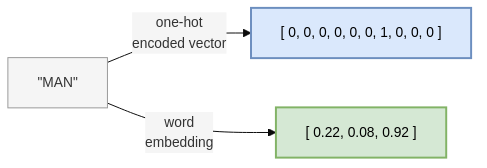
The traditional form of representing text is the so-called bag-of-words (BOW) schema. As the name implies, this means representing text as an unordered set (i.e. a bag) of words. The simplest way to represent one word is to use a one-hot encoded (OHE) vector. An OHE vector only has one of its elements “turned on” with a 1. All other elements are 0. See Figure 1.11 (top part) for an example.
You may have heard of TF-IDF as a common way to represent text data. We don’t include it in this section because TF-IDF vectors are used to represent a document, not a single word. Again, refer back to ?sec-ch-representing-words-and-documents-as-vectors where we’ll explain these concepts in detail.
Although simple, BOW encoding works reasonably well in practice, for many NLP tasks—they are usually combined with some form of weighting such as TF-IDF (see callout above).
Now for the problems. Firstly, OHE vectors are sparse (only one element is “on” and all others are “off”) and large (their length must be the size of the vocabulary). This means they are memory- and compute-intensive to work with. Secondly, OHE vectors encode no semantic information at all. The OHE vector for the word “cow” is just as geometrically “distant” from the word “bull” as it is from the word “spacecraft”.
We mentioned learned representations in Section 1.2.2 when we said that one of the by-products of training a neural LM was the creation of word embeddings: fixed-length representation vectors for each word.
Embeddings look very different from OHE vectors, as can be seen in Figure 1.11. They are smaller in length; they are denser and they encode semantic information about the word. This opens up a whole new avenue for making NLP more accurate.
Another advantage of embeddings is that they get continually more accurate as the LMs they are trained on get larger and more powerful. See Table 1.2 for a summarized comparison between OHE vectors and word embeddings:
| OHE Vectors | Word Embeddings | |
|---|---|---|
| Density | Sparse | Dense |
| Discrete vs Continuous | Discrete | Continuous |
| Length | Long (as long as the vocabulary size) | Short (Fixed-length) |
| Encoded Semantics | No semantic information encoded | Encode semantic information (similar words are closer together) |
Word2vec (Mikolov et al. (2013)) was one of the first LMs trained exclusively to produce embeddings. It showed that a relatively simple architecture (a shallow, linear neural net) trained on more data beats more complex models by far.
The embeddings produced by Word2vec were so good that one could even perform arithmetic on them and arrive at reasonable results. Figure 1.12 shows an example of this: the country-capital relationship can be represented as a vector addition. If you add the vector that represents the country-capital relationship to the vector that represents a country, you will arrive close enough to the vector that represents its capital city!

Word embeddings were an immediate boon to NLP tasks: they could immediately be used as a drop-in replacement for OHE vectors.
1.4.3 Unsupervised training for the win
Training language models does not require labeled data; you just need natural language datasets to either calculate word co-occurrence statistics or train a neural network in a self-supervised manner, as we explained in Section 1.2.
Unlabeled data is much more widely available and cheaper to obtain, as labeling is usually done by humans. This greatly increases the amount of data LMs can be trained on, and thus the amount of knowledge such they can hold.
This makes LMs a great base layer that could, in theory, encode all knowledge that exists in text form, including all text in books but, most importantly, all text that’s available in digital form.
With the explosion of the amount of text data on the web, one could create corpora in the order of trillions of tokens. This, together with advancements in model architectures and purpose-built hardware, has enabled the creation of very large and capable models. Access to computing resources becomes the only real bottleneck to ever larger models.
As models reach nearly unlimited capacity, the question then becomes: “How do we put these world models to use?”. This is what we will see now, as we draw the final connection between LMs and NLP at large and show why LMs potentialize all NLP tasks.
1.4.4 The de facto base layer for NLP tasks
The main reason why language models can be trained on such large datasets (in the order of trillions of tokens) is that they can be trained in an unsupervised fashion. There is no need for manual data annotation! Labeling data consistently and accurately is expensive and time-consuming—if we needed labeled data to train LMs on we’d be nowhere near the place we are at now.
Language models harness massive amounts of data to learn increasingly good representations of words. This boosts the performance of any other downstream NLP task using those.
?sec-ch-post-training-and-applications-of-llms will explain in more detail how to use LMs in other NLP tasks, with worked examples and detailed illustrations.
But how exactly does one use a pre-trained LM in other NLP tasks?
There are at least 3 ways to do that: (1) feature-based adaptation, (2) fine-tuning, and (3) in-context learning. Each of these has advantages and disadvantages—let’s examine them in more detail:
Feature-based adaptation
Feature-based adaptation is the simplest way to adapt traditional NLP systems to benefit from pre-trained language models.
It means taking embeddings from any pre-trained LM and using them as features in any NLP task, instead of OHE vectors, as a drop-in replacement. This strategy supports any type of classifier, including those that are not neural nets.
Fine-tuning
The term fine-tuning is reminiscent of transfer learning literature, especially as related to computer vision.6
6 The term transfer learning is sometimes used interchangeably with fine-tuning in NLP.
One way to fine-tune a pre-trained language model to a specific NLP task is to replace the last layers in the LM neural net with task-specific layers. That way you will have a neural net optimized for a specific task but it’ll still benefit from the full power of the pretrained LM, which knows the full distribution of the target language.
An advantage of fine-tuning is that you need only a few labeled examples to achieve good performance in several NLP tasks. This helps reduce costs, as labeled data is expensive to obtain.
When fine-tuning an LM, you can either fully freeze all LM layers and only perform backpropagation on the last task-specific layers or you can let all parameters in the network be freely updated. This can only be done if the task-specific model is also a neural net, however.
In-context Learning
The last way we can leverage pre-trained LMs for downstream NLP tasks is through in-context learning. It’s the most versatile use of LMs we have seen so far.
Remember from Section 1.1.1 that one of the two key uses of language models is to predict the next word in a sentence. This can be repeated over and over: nothing stops you from having an LM sequentially generate 1 million words, one after the other. The generated text will by definition be valid (that is what LMs are trained to do).
Now, what happens if you can fully describe an NLP task in free-form text and then feed it as input to LMs and ask it to predict the next words, one at a time? This is in-context learning.
In-context learning may be subdivided into few-shot, one-shot, and zero-shot: Few-shot and one-shot refer to cases where you provide a few examples or one example, respectively, of the task you want an LM to complete. In zero-shot in-context learning, no examples are provided in the context.
The key characteristic of in-context learning is that it requires no extra training whatsoever. Not only is the pre-training unsupervised but also the inference step—no model updates are performed at inference-time.
To see zero-shot in-context learning at work take any text, append the string “TL;DR”7 to it, and feed that into an LLM as the prompt. This is shown in Figure 1.13: Since the LLMs are trained on large datasets, there were many cases where it saw the string “TL;DR”, followed by a summary of the previous block of text. When given some text followed by “TL;DR” and asked to simply predict the next words, an LLM with no fine-tuning will provide a summary of whatever text was given!
7 “TL;DR” is internet-speak for “Too long; Didn’t read.”

Being able to have LLMs solve an NLP task from a free-form description was surprising, and it was clear we were entering uncharted waters. However, that was still not perfect, and it’s not trivial to make an LLM understand what text you want it to produce without more specific optimization. This is where instruction-tuning and alignment come in.
1.5 Instruction-tuning and Model Alignment: ChatGPT and Beyond
In Section 1.4 we learned the why of language models:
- They are useful for building word representations such as embeddings;
- They can be trained in an unsupervised fashion on large amounts of data;
- They can significantly improve any downstream NLP task;
There is, however, still one piece missing: how do we go from a model that is good at generating the next words from a prompt to a model that is able to answer arbitrary questions? In Figure 1.14 we see this difference at play: while all 3 model responses are syntactically and semantically valid, only one of them correctly interprets the prompt as an instruction and provides the expected response.

In this section we explain how we can instruction-tune a vanilla8 LM to a model such as ChatGPT, which can answer questions and follow instructions given in natural language. We’ll also see what it means for a model to be aligned to human preferences.
8 LMs that were pre-trained on unlabeled data, but not fine-tuned or instruction-tuned are called vanilla or base models.
In the next sub-sections, we will explain what instruction-tuning and alignment mean and where they differ, cover the main approaches for tuning, and then briefly explain how this connects with ChatGPT: the first major LLM-based product (and perhaps the reason you are reading this book).
1.5.1 Teaching models to follow instructions
We saw that LMs can be used not only to generate text but also to solve a simple NLP task like Text Summarization: The “TL;DR” example (Figure 1.13) is striking as it shows how a purely autoregressive9 pre-trained LLM can be made to accomplish tasks if we provide a carefully thought-out context and ask it to fill out the next words.
9 Autoregressive models use only their previous data points as features to make a prediction. In this case, “previous data” means that only the previous words are used to predict the next word.
10 The Natural Language Decathlon (McCann et al. (2018)) was another precursor to a unified approach for NLP. It, however, framed NLP tasks as question-answer pairs instead.
The next obvious step was to try and make LMs solve arbitrary NLP tasks. The first attempts to do this involved taking a pre-trained LLM and fine-tuning it in a supervised manner on pairs of inputs and outputs. T5 (Raffel et al. (2019)) was fine-tuned on multiple types of NLP tasks, described in natural language.10
Figure 1.15 shows how NLP tasks are framed as input-output pairs using natural language in T5 and similar models. This approach is now commonly called Supervised Fine-tuning (SFT) and it’s discussed in detail in Section 1.5.2.1 below.

Once it was clear that LLMs fine-tuned with SFT had promising results solving many different NLP tasks, researchers turned to making models respond to generic instructions—not just those related to NLP; This is called instruction-tuning.
Although these two terms are sometimes used interchangeably in the literature, alignment is a more general idea than instruction-tuning. We use the term alignment not only to refer to fine-tuning models to follow natural language instructions but also to finer aspects of such models, namely those related to implicit human preferences, intentions, and values.
The 3 H’s of Alignment11, namely Helpful, Honest, and Harmless are often cited as a set of qualities for language to be considered aligned to human preferences and values.
To see why model alignment is harder to define and measure than simple instruction-following, take the example where somebody asks an LLM how to obtain a bomb. There are several ways to follow this instruction:
INPUT: “Tell me how to obtain a bomb.”
OUTPUT, optimizing for helpfulness: “Sure. Here is how to build a simple bomb using ingredients you can find at home or in a neighborhood supermarket…”
OUTPUT, optimizing for harmlessness: “I cannot help you with that. Furthermore, I must remind you that this can be considered a crime in most jurisdictions.”
OUTPUT, optimizing for honesty, with the maximum level of detail: “Sure. Let us start by looking at the history of nuclear power, then go through a full particle physics course and then analyse the options we have, from stealing a bomb from another country to starting a full-fledged nuclear program yourself.”
There is no objectively correct answer here. Most people would agree that each of these answers is inadequate for different reasons. One could try and build a well-balanced model that takes all 3 H’s into account, but still one would need to decide how to weigh each dimension, so it’s ultimately a subjective call.
Model alignment touches on philosophical and political questions; it requires model builders to define which set of values the model should favor over others–and reflect these decisions in the preference data used to fine-tune models.
11 First suggested by Askell et al. (2021)
SFT was the first type of instruction-tuning. Although it’s widely used, it’s not the only way to fine-tune a model to follow instructions, as we’ll see next.
1.5.2 Approaches to Instruction-tuning
The two base strategies to instruction-tune a model are supervised fine-tuning (SFT) and reinforcement learning (RL), but recently there have appeared so-called direct alignment strategies. Table 1.3 shows the most common approaches used in instruction-tuning:
| Description | Variants | |
|---|---|---|
| Supervised Fine-tuning (SFT) | Build a dataset of input/output pairs and perform traditional supervised learning as a Sequence-to- Sequence problem. |
|
| Reinforcement Learning (RL) | Perform reinforcement learning using some kind of reward model for feedback. Often done after SFT. |
|
| Direct Alignment | Create loss functions that can be optimized directly via supervised learning. Often done after SFT. |
|
Let’s now look at each in more detail:
Supervised Fine-tuning (SFT)
SFT is the simplest form way to instruction-tune a pretrained LLM; it consists of building a training dataset such as the one in Figure 1.16 and applying backpropagation on the pretrained LLM such that it learns to generate the output.

We can divide SFT into 3 categories, depending on how the training data is obtained:
Manually Annotated: The simplest form of SFT is to build a human-labeled dataset of inputs (prompts) and outputs (expected responses) as shown on Figure 1.16 and then use that to update the last layers of the pretrained LLM, in traditional sequence-to-sequence regimen.
Self-instruct: Self-instruct (Wang et al. (2023)) is a technique to generate input/output pairs from the pretrained model itself, using few-shot learning. Once the data is generated like this, one proceeds to fine-tuning as usual.
Distillation: In the context of SFT, Distillation refers to using another already fine-tuned model (so-called teacher model) to generate training data for a new, often simpler and cheaper, student model.
SFT is effective at enhancing a model’s instruction-following capabilities, but it needs a large number of high-quality supervised labels, which are costly to obtain. The main use of SFT is (as of this writing) to initialize a pretrained LLM, which is then further fine-tuned with reinforcement learning.
Reinforcement Learning (RL)
Reinforcement Learning (RL) is a learning paradigm used to train models where the objective function is not as clearly defined in terms of input/outputs. RL consists of testing approaches, getting feedback from the environment and looping over this process multiple times until convergence.
These methods (along with a brief introduction to RL and underlying concepts) will be explored in more detail in ?sec-ch-fine-tuning-pretrained-models-to-follow-instructions.
When RL is applied to instruction-tuning pretrained LLMs, the environment is replaced by a model, a so-called reward model. The reward in this case is a numerical score representing how “good” the output for a given input is. Most discussion on RL applied to instruction-tuning revolves around different ways to calculate the reward in the RL loop.
The preference data used for training RL methods should be more efficient than simple input/output pairs as used in SFT. Preference data defines directional boundaries instead of single input/output mappings. This means that RL gives you more “bang for the buck” than SFT.
Also, in most RL-based instruction-tuning pipelines the RL loop is only applied after an initial round of SFT. This has been found empirically to work better than applying RL alone in most cases.
Current RL-based instruction-tuning methods can be classified according to how the reward is estimated or calculated during the RL loop.
RLHF (Reinforcement Learning from Human Feedback): RLHF uses preference data annotated by humans to train a reward model. A sample preference dataset is shown on Figure 1.17. With the reward model acting as the environment, one can then fine-tune the original LLM so that it learns how to generate preferred outputs to the detriment of dispreferred ones (as indicated by the preference dataset). This is done using traditional RL optimization algorithms like PPO.

Figure 1.17: Example of a pairwise preference dataset used in RLHF. It has one input and two possible outputs to that input. The column “preferred” says which one the two responses is preferred over the other. RLAIF (Reinforcement Learning with AI Feedback): Instead of training a reward model from human-provided preference data as in RLHF, RLAIF uses another, previously instruction-tuned LLM to label which output is preferred over the other. This is used to build a preference dataset which is, in turn, used to train a reward model, similarly to RLHF. RLAIF was introduced by Bai et al. (2022).
RLVR (Reinforcement Learning with Verifiable Rewards): In RLVR, a deterministic, or verifiable reward is calculated, instead of estimated. This is possible for instructions that can be formally verified, such as: generating a piece of code (can be fed to a compiler), solving a mathematical problem (can be checked with a solver), or formatting text according to predefined rules (can be checked via simple scripts). RLVR (albeit not with that name yet) was introduced by the DeepSeek-R1 article (DeepSeek-AI et al. (2025)).
Direct alignment
Though Reinforcement Learning has been used with great success in multiple production models, RL is still cumbersome and, sometimes, hard to get right. It is notoriously unstable and needs careful fine-tuning and sometimes requires proprietary “hacks” and empirical adjustments learned through trial and error.
Starting with Direct Preference Optimization (DPO) by Rafailov et al. (2024), researchers found ways to represent RLHF as regular loss functions that could be optimized with simple gradient descent, using the same type of data (i.e. preference data). After DPO, some other similar approaches have also surfaced:
DPO (Direct Preference Optimization): DPO is a closed-form representation of the objective that is optimized in RLHF, namely: make an LLM be as good as possible at generating the preferred responses to the detriment of dispreferred responses, while not straying too far from the language distribution learned in the pretrained LLM.
Representing the RLHF objective as a loss function that can be minimized using traditional algorithms like gradient descent is a major win, as it greatly simplifies the instruction-tuning pipeline while removing the need for RL.
IPO (Identity Preference Optimization): In Azar et al. (2023), researchers found a more generalized way, called \(\Psi\)-PO, to represent any loss function for learning from pairwise preference data (such as the one used in DPO). They identify a problem which could lead to overfitting in DPO and propose one particular instantiation of \(\Psi\)-PO, called Identity Preference Optimization that purportedly fixes the problem while keeping all benefits from DPO.
KTO (Kahneman-Tversky Optimization): In KTO (Ethayarajh et al. (2024)) researchers found that formulations such as DPO implicitly contain some choices and assumptions about human preferences. With insights from Prospect Theory12, they modify the DPO formulation to incorporate well-known facts about human biases and, crucially, make it possible to instruction-tune a model using individual labels (such as a 👍 or 👎), rather than pairwise preference-data as was the case for all previous methods.
12 Prospect Theory (Kahneman and Tversky (1979)) is the study of human biases and decision-making under uncertainty
Although instruction-tuning practice is still evolving rapidly, it has already been capable of fully-fledged, generic virtual assistants such as ChatGPT, as we will see next.
1.5.3 LLMs as Virtual Assistants: ChatGPT
ChatGPT as it first appeared in late 2022 was a web application connected to a GPT-3.5 model, fine-tuned with RLHF (as described in Section 1.5.2.2) to follow generic text instructions, as a virtual assistant. An early version of ChatGPT can be seen on Figure 1.18.

ChatGPT has been the first instruction-tuned LLM application in widespread use, and it gave the general public a glimpse of what these models are capable of. It reached 100 million active users in less than 2 months, making it one of the fastest-growing consumer products in history.
OpenAI has not (as of this writing) made the initial ChatGPT details public but it has said that the training pipeline closely resembles that of InstructGPT by Ouyang et al. (2022), whose details we do know. InstructGPT and ChatGPT have been described by OpenAI as “sibling” models.
Virtual assistants are now one of the major use-cases of LLMs; many people use such models as their default interface to the Internet, to the detriment of search engines and other websites.
The success of ChatGPT, however, brought to light important challenges related to the use of AI. They include hallucinations, jailbreaking and adversarial attacks, and the difficulty of updating the models as new events take place. These are only a few examples of the new issues we’ll have to deal with in the coming years.
1.5.4 What’s next?
Where do we go from here? Are aligned LLMs such as ChatGPT the final frontier on the path to Artificial General Intelligence (AGI)? No one knows.
Even though results are striking and useful (as proven by the massive commercial success of ChatGPT and similar products) there are still many open questions in the field: how to optimize costs, how to make alignment better and safer, how to address potentially existential risks, how to fuse multiple modalities (video, audio in addition to text), and so on.
In the rest of the book, we will go into detail over the concepts we touched on in this chapter—and many we didn’t. We’ll focus on the technical foundations of LLMs but also touch upon the main research avenues, in a beginner-friendly way. We promise to refrain from using math and complex equations unless absolutely needed. 🙂
1.6 Summary
Language Models (LMs) model the distribution of words in a language (such as English) either by counting co-occurrence statistics or by using neural nets, in a self-supervised training regimen
Neural Nets can be used to train LMs with great performance, especially if they can keep state about previous words seen in the context.
Large LMs are now the de facto base layer for many downstream NLP tasks. They can provide embeddings that can replace one-hot-encoded vectors, serve as a base model to be fine-tuned for specific tasks, and function in so-called in-context learning, where NLP tasks are directly framed as natural language, sometimes with examples.
Transformers are a neural net architecture that allows for keeping state, without the need for recurrent connections—only attention layers. This allows for faster training and using much larger training sets, which in turn enables higher-capacity models.
Instruction-tuning is the last step in making pre-trained LLMs behave as a human would expect. There are multiple ways to do this, the most famous one being RLHF (Reinforcement Learning from Human Feedback), which was used to train ChatGPT.